One-way ANOVA (Analysis of Variance) is a statistical test used to compare the means of three or more samples to determine if there are significant differences among them. It is based on the assumption that the samples are drawn from normally distributed populations with equal variances.
Steps in One-way ANOVA:
- Specify the null and alternative hypotheses. The null hypothesis is usually that there is no difference among the means of the samples, while the alternative hypothesis is that there is at least one difference among the means of the samples.
- Select three or more samples from the populations and calculate the sample means and sizes.
- Calculate the overall mean of all the samples combined.
- Calculate the sum of squares within groups (SSW), the sum of squares between groups (SSB) and the degrees of freedom for both SSW and SSB.
- Calculate the F statistic as the ratio of the Mean SSB to the Mean SSW.
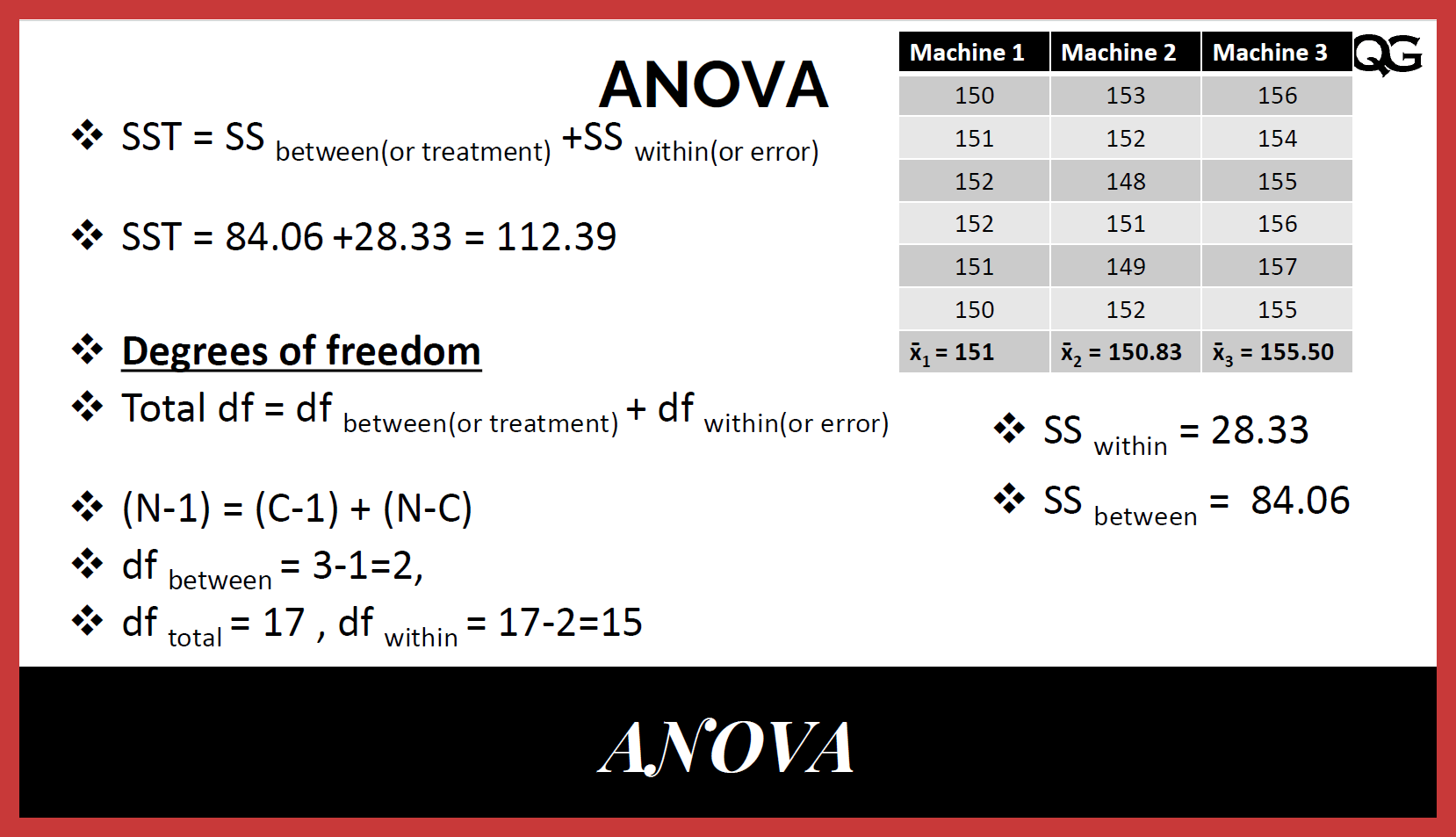
- Determine the critical value of the F statistic based on the test's significance level (alpha) and the degrees of freedom for the numerator and denominator. The degrees of freedom for the numerator is the number of groups minus 1, while the degrees of freedom for the denominator is the total sample size minus the number of groups.
- Compare the calculated F statistic to the critical value to determine whether to reject or fail to reject the null hypothesis. If the calculated F statistic exceeds the critical value, the null hypothesis is rejected, and the alternative hypothesis is accepted.
Conditions for One-way ANOVA:
To conduct a valid one-way ANOVA, the following conditions must be met:
- The samples must be drawn randomly from the populations.
- Each observation in each sample must be independent of the others.
- The population distributions must approximate a normal distribution.
- The population variances must be equal.
Typical Null and Alternate Hypotheses in One-way ANOVA:
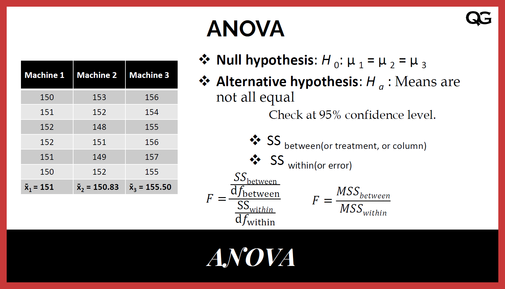
The null hypothesis in a one-way ANOVA is that there is no difference among the means of the samples. This can be expressed as:
H0: μ1 = μ2 = … = μk
Where μ1, μ2, …, μk are the means of the samples.
The alternate hypothesis is the opposite of the null hypothesis and is that there is at least one difference among the means of the samples. This can be expressed as:
Ha: At least one μi ≠ μj
Calculating SSW and SSB:
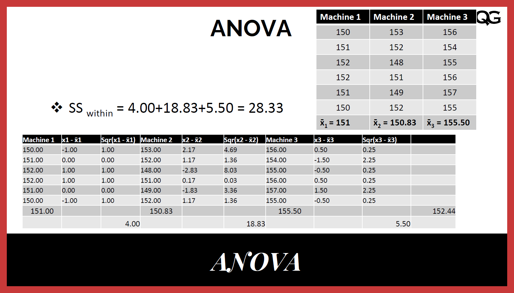
Sum of Square Within (SSW):
The Sum of Squares Within (SSW) measures the variance within the groups. It is calculated as the sum of the squared differences between each individual observation and the group mean divided by the degrees of freedom within the groups.
The formula for calculating SSW is:
$$SSW = Σ(X_i - M)^2$$
Where X is the individual observation, and M is the group mean.

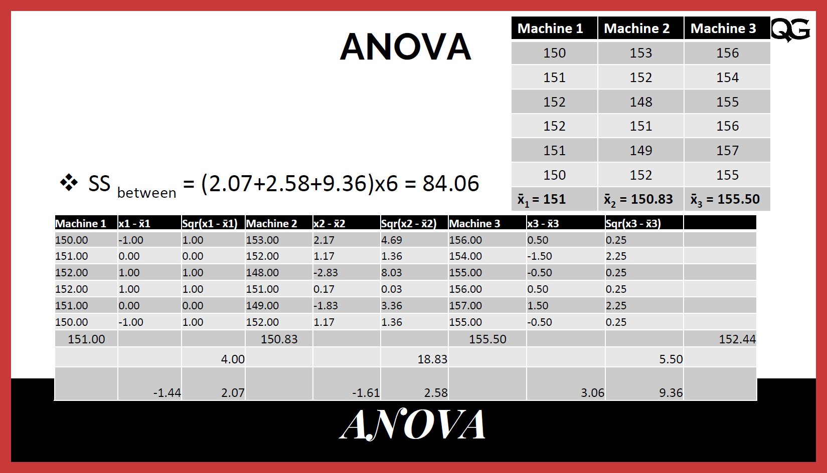
Sum of Square Between (SSB):
The formula for calculating the Sum of Squares Between (also known as SSB) is:
$$SSB = Σ(Mi - M)^2 * n_i$$
Where Mi is the mean of the ith group, M is the grand mean (the mean of all observations), and n is the number of observations in each group. (assuming an equal number of observations in each group)
To calculate SSB, you would first need to find the mean of each group and the grand mean. Then, for each group, you would subtract the grand mean from the group mean and square the result. Finally, you would multiply this squared difference by the number of observations in the group and sum the results for all groups to get the SSB.

Calculating F Statistic:
The F statistic in a one-way ANOVA (analysis of variance) is a measure of how much variation in the data can be attributed to the different groups (also known as "treatments") compared to the variation within the groups. It is calculated as the ratio of the Mean SSB (mean sum of squares between groups) to the Mean SSW (mean sum of squares within groups).
The Mean SSB is a measure of the variation between the group means, and is calculated as:
$$Mean SSB = \frac{SSB}{(k-1)}$$
Where SSB is the sum of squares between groups, and k is the number of groups.
The Mean SSW is a measure of the variation within each group, and is calculated as:
$$Mean SSW = \frac{SSW}{(n-k)}$$
Where SSW is the sum of squares within groups, and n is the total number of observations.
The F statistic is then calculated as:
$$F = \frac{Mean SSB}{Mean SSW} = \frac{\frac{SSB}{k-1}}{\frac{SSW}{n-k}}$$
A high F value indicates that there is a significant difference between the group means, while a low F value indicates that the group means are not significantly different. The F statistic is used to test the null hypothesis that there is no significant difference between the group means. If the calculated F value is greater than the critical F value, the null hypothesis is rejected, and it is concluded that there is a significant difference between the group means.
Calculating Critical Values:
The critical values for the F statistic in a one-way ANOVA depend on the significance level of the test and the degrees of freedom for the numerator and denominator. The degrees of freedom for the numerator are the number of groups minus 1 or (k-1), while the degrees of freedom for the denominator are the total sample size minus the number of groups or (n-k). Using these two values (significance level and degrees of freedom), you can find out the value of the critical F statistic using an F Distribution Table.

In addition, you can use statistical software to find out the critical value. In Excel, you can use =F.INV.RT(probability, deg_freedom1, deg_freedom2) for the right tail value.
Remember: One-way ANOVA is always a one-tail (right tail) test.

